[ < ] | [ > ] | [ << ] | [ Up ] | [ >> ] | [Top] | [Contents] | [Index] | [ ? ] |
8.1 Introduction to Plotting | ||
8.2 Plotting Formats | ||
8.3 Functions and Variables for Plotting | ||
8.4 Plotting Options | ||
8.5 Gnuplot Options | ||
8.6 Gnuplot_pipes Format Functions |
[ < ] | [ > ] | [ << ] | [ Up ] | [ >> ] | [Top] | [Contents] | [Index] | [ ? ] |
Maxima uses an external plotting package to make the plots (see the
section on Plotting formats). The plotting functions calculate a set of
points and pass them to the plotting package together with a set of
commands. That information can be passed to the external program either
through a pipe or by calling the program with the name of a file where
the data has been saved. The data file is given the name
maxout.interface
, where interface
is the name of the
plotting interface being used (gnuplot, xmaxima, mgnuplot or
gnuplot_pipes).
The maxout.interface
file, in the cases when it is used, is
created in the directory specified by the system variable
maxima_tempdir. That location can be changed; by assigning to that
variable a string that represents a valid directory where Maxima can
create new files.
After a plot has been created, the file maxout.interface
can be
executed again with the appropriate external program. If a Maxima plotting
command fails to show anything, that file can be inspected to look for
possible sources of problems.
Categories: Plotting
[ < ] | [ > ] | [ << ] | [ Up ] | [ >> ] | [Top] | [Contents] | [Index] | [ ? ] |
There are currently two external plotting programs that Maxima use: Gnuplot
and Xmaxima. There are various different formats for those programs,
which can be selected with the option plot_format
(see
the Plotting Options section).
The plotting formats are the following:
Used to launch the external program gnuplot, which must be installed in
your system. All plotting commands and data are saved into the file
maxout.gnuplot
.
This format is not available in Windows platforms.
It is similar to the gnuplot
format except that the commands are sent
to gnuplot through a pipe, while the data are saved into the file
maxout.gnuplot_pipes
. A single gnuplot process is kept open
and subsequent plot commands will be sent to the same process, replacing
previous plots, unless the gnuplot pipe is closed with the function
gnuplot_close()
. When this format is used, the function
gnuplot_replot
can be used to modify a plot that has already
displayed on the screen (see gnuplot_replot
).
This format should only be used to plot to the
screen; for plotting to files it is better to use the gnuplot
format.
Mgnuplot is a Tk-based wrapper around gnuplot. It is included in the Maxima distribution. Mgnuplot offers a rudimentary GUI for gnuplot, but has fewer overall features than the plain gnuplot interface. Mgnuplot requires an external gnuplot installation and, in Unix systems, the Tcl/Tk system.
Xmaxima is a Tcl/Tk graphical interface for Maxima that can also be used
to display plots created when Maxima is run from the console or from other
graphical interfaces. To use this format, the xmaxima program, which is
distributed together with Maxima, should be installed. If Maxima is
being run from xmaxima itself, this format will make the plot functions
send the data and commands through the same socket used for the
communication between Maxima and Xmaxima. When used from the console
or from other interface, the commands and data will be saved in the file
maxout.xmaxima
, and the xmaxima program will be launched with the
name of the location of that file as argument.
In previous versions this format used to be called openmath
; that
old name will still be accepted as a synonym for xmaxima
.
Categories: Plotting
[ < ] | [ > ] | [ << ] | [ Up ] | [ >> ] | [Top] | [Contents] | [Index] | [ ? ] |
It plots the contours (curves of equal value) of expr
over the region x_range by y_range.
Any additional arguments are treated the same as in plot3d
.
This function only works when the plot format is either gnuplot
or gnuplot_pipes
. The additional package implicit_plot
can
also be used to plot contours and it works for any format. See
implicit_plot
.
Examples:
(%i1) contour_plot (x^2 + y^2, [x, -4, 4], [y, -4, 4])$
(%i1) F(x, y) := x^3 + y^2; 3 2 (%o1) F(x, y) := x + y (%i2) contour_plot (F, [u, -4, 4], [v, -4, 4])$
You can add any options accepted by plot3d
; for instance, the
option legend
with a value of false, to remove the
legend. Gnuplot chooses, by default, 3 contours to show. to increase the
number of levels, it is necessary to specify a custom gnuplot preamble:
(%i1) contour_plot (u^3 + v^2, [u, -4, 4], [v, -4, 4], (%i2) [legend,false], [gnuplot_preamble,"set cntrparam levels 12"])$
Categories: Plotting
Returns a value of the option with name keyword, stored in the
global variable plot_options
. A value of 1 for the index will
return the keyword itself; a value of 2 turn returns the first parameter
following the keyword, and so on.
See also plot_options
, set_plot_option
and the section on
Plotting Options.
Returns a function suitable to be used in the option transform_xy
of plot3d. The three variables var1, var2, var3 are
three dummy variable names, which represent the 3 variables given by the
plot3d command (first the two independent variables and then the
function that depends on those two variables). The three functions
fx, fy, fz must depend only on those 3 variables, and
will give the corresponding x, y and z coordinates that should be
plotted. There are two transformations defined by default:
polar_to_xy
and spherical_to_xyz
; see the documentation
for those two transformations.
Categories: Plotting
It can be given as value for the transform_xy
option of
plot3d. Its effect will be to interpret the two independent variables in
plot3d as the distance from the z axis and the azimuthal angle (polar
coordinates), and transform them into x and y coordinates.
Categories: Plotting
Where plot, plot_1, ..., plot_n can be either
expressions, function names or a list with
the any of the forms: [discrete, [x1, ..., xn],
[y1, ..., yn]]
, [discrete, [[x1, y1],
..., [xn, ..., yn]]
or [parametric, x_expr,
y_expr, t_range]
.
Displays a plot of one or more expressions as a function of one variable or parameter.
plot2d
displays one or several plots in two dimensions. When
expressions or function name are used to define the plots,
they should all depend on only one variable var and the use of
x_range will be mandatory, to provide the name of the variable and
its minimum and maximum values; the syntax for x_range is:
[variable, min, max]
.
A plot can also be defined in the discrete or parametric forms. The discrete form is used to plot a set of points with given coordinates. A discrete plot is defined by a list starting with the keyword discrete, followed by one or two lists of values. If two lists are given, they must have the same length; the first list will be interpreted as the x coordinates of the points to be plotted and the second list as the y coordinates. If only one list is given after the discrete keyword, each element on the list should also be a list with two values that correspond to the x and y coordinates of a point.
A parametric plot is defined by a list starting with the keyword
parametric, followed by two expressions or function names and a
range for the parameter. The range for the parameter must be a list with
the name of the parameter followed by its minimum and maximum values:
[param, min, max]
. The plot will show the path
traced out by the point with coordinates given by the two expressions or
functions, as param increases from min to max.
A range for the vertical axis is an optional argument with the form:
[y, min, max]
(the keyword y is always used for
the vertical axis). If that option is used, the plot will show that
exact vertical range, independently of the values reached by the plot.
If the vertical range is not specified, it will be set up according to
the minimum and maximum values of the second coordinate of the plot
points.
All other options should also be lists, starting with a keyword and
followed by one or more values. See plot_options
.
If there are several plots to be plotted, a legend will be written to identiy each of the expressions. The labels that should be used in that legend can be given with the option legend. If that option is not used, Maxima will create labels from the expressions or function names.
Examples:
Plot of a common function:
(%i1) plot2d (sin(x), [x, -%pi, %pi])$
If the functions grows too fast, it might be necessary to limit the values in the vertical axis using the y option:
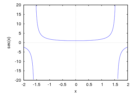
(%i1) plot2d (sec(x), [x, -2, 2], [y, -20, 20])$ plot2d: some values were clipped.
The aspect of the plot might be different depending on the plotting program used. For instance, when the plot box is disable, Xmaxima will plot the axes using arrows:
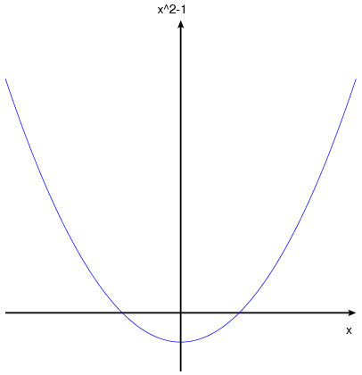
(%i1) plot2d ( x^2-1, [x, -3, 3], [y, -2, 10], [box, false], [plot_format, xmaxima])$
A plot with a logarithmic scale:
(%i1) plot2d (exp(3*s), [s, -2, 2], [logy])$
Plotting functions by name:
(%i1) F(x) := x^2 $ (%i2) :lisp (defun |$g| (x) (m* x x x)) $g (%i2) H(x) := if x < 0 then x^4 - 1 else 1 - x^5 $ (%i3) plot2d ([F, G, H], [u, -1, 1], [y, -1.5, 1.5])$
A plot of the butterfly curve, defined parametrically:
(%i1) r: (exp(cos(t))-2*cos(4*t)-sin(t/12)^5)$ (%i2) plot2d([parametric, r*sin(t), r*cos(t), [t, -8*%pi, 8*%pi], [nticks, 2000]])$
A "circle" with two turns, when plotted with only 7 points:
(%i1) plot2d ([parametric, cos(t), sin(t), [t, -2*%pi, 2*%pi], [nticks, 8]])$
Plot of a common function together with the parametric representation of a circle. The size of the plot has been adjusted with the x and y options, to make the circle look round and not deformed as an ellipse. These values work well for the Postscript terminal used to produce this plot; you might have to adjust the values for your screen.
(%i1) plot2d([[parametric, cos(t), sin(t) ,[t,0,2*%pi], [nticks, 80]], abs(x)], [x,-2,2], [y, -1.5, 1.5])$ plot2d: some values were clipped.
A plot of a discrete set of points, defining x and y coordinates separately:
(%i1) plot2d ( [ discrete, [10, 20, 30, 40, 50], [.6, .9, 1.1, 1.3, 1.4]] )$
The same points shown in the previous example, defining each point separately and without any lines joining the points:
(%i1) plot2d([discrete, [[10, .6], [20, .9], [30, 1.1], [40, 1.3], [50, 1.4]]], [style, points])$
In this example, a table with three columns is saved in a file "data.txt" which is then read and the second and third column are plotted on the two axes:
(%i1) with_stdout ("data.txt", for x:0 thru 10 do print (x, x^2, x^3))$ (%i2) data: transpose ( read_matrix ("data.txt"))$ (%i3) plot2d ([discrete, data[2], data[3]], [style,points], [point_type,diamond], [color,red])$
A plot of experimental data points together with the theoretical function that predicts the data:
(%i1) xy: [[10, .6], [20, .9], [30, 1.1], [40, 1.3], [50, 1.4]]$ (%i2) plot2d([[discrete, xy], 2*%pi*sqrt(l/980)], [l,0,50], [style, points, lines], [color, red, blue], [point_type, asterisk], [legend, "experiment", "theory"], [xlabel, "pendulum's length (cm)"], [ylabel, "period (s)"])$
See also the section about Plotting Options.
Categories: Plotting
Displays a plot of one or more surfaces defined as functions of two variables or in parametric form.
The functions to be plotted may be specified as expressions or function names. The mouse can be used to rotate the plot looking at the surface from different sides.
Examples:
Plot of a common function:
(%i1) plot3d (2^(-u^2 + v^2), [u, -3, 3], [v, -2, 2])$
Use of the z option to limit a function that goes to infinity (in this case the function is minus infinity on the x and y axes); this also shows how to plot with only lines and no shading:
(%i1) plot3d ( log ( x^2*y^2 ), [x, -2, 2], [y, -2, 2], [z, -8, 4], [palette, false], [color, magenta, blue])$
The infinite values of z can also be avoided by choosing a grid that does not fall on any asymptotes; this example also shows how to select one of the predefined palettes, in this case the fourth one:
(%i1) plot3d(log(x^2*y^2), [x, -2, 2], [y, -2, 2], [grid, 29, 29], [palette, get_plot_option(palette,5)])$
Two surfaces in the same plot, sharing the same domain; in gnuplot the two surfaces will use the same palette:
(%i1) plot3d ( [2^(-x^2 + y^2), 4*sin(3*(x^2+y^2))/(x^2+y^2), [x, -3, 3], [y, -2, 2]])$
The same two surfaces, but now with different domains; in xmaxima each surface will use a different palette, chosen from the list defined by the option palette:
(%i1) plot3d ( [[2^(-x^2 + y^2),[x,-2,2],[y,-2,2]], 4*sin(3*(x^2+y^2))/(x^2+y^2), [x, -3, 3], [y, -2, 2]], [plot_format,xmaxima])$
Plot of a Klein bottle, defined parametrically:
(%i1) e_1: 5*cos(x)*(cos(x/2)*cos(y)+sin(x/2)*sin(2*y)+3.0)-10.0$ (%i2) e_2: -5*sin(x)*(cos(x/2)*cos(y)+sin(x/2)*sin(2*y)+3.0)$ (%i3) e_3: 5*(-sin(x/2)*cos(y)+cos(x/2)*sin(2*y))$ (%i4) plot3d ([e_1, e_2, e_3], [x, -%pi, %pi], [y, -%pi, %pi], [grid, 40, 40])$
Plot of a spherical harmonic, using of the predefined transformations,
spherical_to_xyz
, to transform from spherical to rectangular
coordinates. See the documentation for spherical_to_xyz
.
(%i1) plot3d (sin(2*theta)*cos(phi), [theta,0,%pi], [phi,0,2*%pi], [transform_xy, spherical_to_xyz], [grid,30,60])$
Use of the predefined function polar_to_xy
to transform from
cylindrical to rectangular coordinates. See the documentation for
polar_to_xy
. This example also shows how to eliminate the
bounding box and the legend.
(%i1) plot3d(r^.33*cos(th/3), [r,0,1], [th,0,6*%pi], [grid,12,80], [transform_xy, polar_to_xy], [box, false], [legend,false])$
Plot of a sphere using the transformation from spherical to rectangular coordinates. In xmaxima the three axes are scaled in the same proportion, maintaining the symmetric shape of the sphere. A palette with different shades of a single color is used:
(%i1) plot3d (5, [theta, 0, %pi], [phi, 0, 2*%pi], [transform_xy, spherical_to_xyz], [plot_format,xmaxima], [palette,[value,0.65,0.7,0.1,0.9]])$
Definition of a function of two-variables using a matrix. Notice the single quote in the definition of the function, to prevent plot3d from failing when it realizes that the matrix will require integer indices.
(%i1) M: matrix([1,2,3,4], [1,2,3,2], [1,2,3,4], [1,2,3,3])$ (%i2) f(x, y) := float('M [round(x), round(y)])$ (%i3) plot3d (f(x,y), [x, 1, 4], [y, 1, 4], [grid, 4, 4])$ apply: subscript must be an integer; found: round(x)
By setting the elevation equal to zero, a surface can be seen as a map
in which each color represents a different level. The option
colorbox
is used to show the correspondence among colors and
levels, and the mesh lines are disabled to make the colors easier to see.
(%i1) plot3d (cos (-x^2 + y^3/4), [x, -4, 4], [y, -4, 4], [mesh_lines_color, false], [elevation, 0], [azimuth, 0], [colorbox, true], [grid, 150, 150])$
See also the section about Plotting Options.
Categories: Plotting
Elements of this list state the default options for plotting.
If an option is present in a plot2d
or plot3d
call,
that value takes precedence over the default option.
Otherwise, the value in plot_options
is used.
Default options are assigned by set_plot_option
. There are other
local options specific to each plotting command, and not included in
this list of global options.
Each element of plot_options
is a list of two or more items. The
first item is the name of the option, and the remainder comprises the
value or values assigned to the option. In some cases, the assigned
value is a list, which may include several items.
See also set_plot_option
, get_option
and the section on
Plotting Options.
Categories: Plotting
Accepts most of the options listed in the section Plotting Options, and
saves them into the global variable plot_options
.
set_plot_option
evaluates its argument and returns the complete
list plot_options
(after modifying the option given).
See also plot_options
, get_option
and the section on
Plotting Options.
Example:
Modification of the grid
values.
(%i1) set_plot_option ([grid, 30, 40]); (%o1) [[t, - 3, 3], [grid, 30, 40], [transform_xy, false], [run_viewer, true], [axes, true], [plot_format, gnuplot_pipes], [color, blue, red, green, magenta, black, cyan], [point_type, bullet, circle, plus, times, asterisk, box, square, triangle, delta, wedge, nabla, diamond, lozenge], [palette, [hue, 0.25, 0.7, 0.8, 0.5], [hue, 0.65, 0.8, 0.9, 0.55], [hue, 0.55, 0.8, 0.9, 0.4], [hue, 0.95, 0.7, 0.8, 0.5]], [gnuplot_term, default], [gnuplot_out_file, false], [nticks, 29], [adapt_depth, 5], [gnuplot_preamble, ], [gnuplot_default_term_command, set term pop], [gnuplot_dumb_term_command, set term dumb 79 22], [gnuplot_ps_term_command, set size 1.5, 1.5;set term postscript \ eps enhanced color solid 24], [plot_realpart, false]]
Categories: Plotting
It can be given as value for the transform_xy
option of
plot3d. Its effect will be to interpret the two independent variables
and the function in plot3d as the spherical coordinates of a point
(first, the angle with the z axis, then the angle of the xy projection
with the x axis and finally the distance from the origin) and transform
them into x, y and z coordinates.
Categories: Plotting
[ < ] | [ > ] | [ << ] | [ Up ] | [ >> ] | [Top] | [Contents] | [Index] | [ ? ] |
All options consist of a list starting with one of the keywords in this section, followed by one or more values. Most of the options can be used in any of the plotting commands (plot2d, plot3d, contour_plot, implicit_plot) or in the function set_plot_option; the exceptions will be specified in the following list.
The maximum number of splittings used by the adaptive plotting routine.
Default value: 5
Categories: Plotting
Where symbol can be either true
, false
, x
or
y
. If false
, no axes will be shown; if equal to x
or y
only the x or y axis will be shown, and if it is equal to
true
, both axes will be shown. This option is used only by plot2d
and implicit_plot.
Default value: true
Categories: Plotting
A plot3d plot can be thought of as starting with its x and y axis
in the horizontal and vertical axis, as in plot2d, and the z axis
coming out of the paper perpendicularly. The z axis is then rotated
around the x axis an angle equals to elevation
and then the xy
plane is rotated around the new z axis an angle azimuth
. This
option sets the value for the azimuth, in degrees.
Default value: 30
See also elevation
.
Categories: Plotting
If set to true
, a bounding box will be drawn for the plot; if set
to false
, no box will be drawn.
Default value: true
Categories: Plotting
In plot2d and implicit_plot, it defines the color (or colors) for the various curves. In plot3d, it defines the colors used for the mesh lines of the surfaces, when no palette is being used; one side of the surface will have color color_1 and the other color_2 (or the same color if there is only one color).
If there are more curves or surfaces than colors, the colors will be repeated in sequence. When using gnuplot, the colors could be: blue, red, green, magenta, black, cyan or black; in xmaxima the colors can be those or a string starting with the character # and followed by six hexadecimal digits: two for the red component, two for green component and two for the blue component. If given the name of an unknown color, black will be used instead.
Default value: blue, red, green, magenta, black, cyan
Categories: Plotting
Where symbol can be either true
or false
. If
true
, whenever plot3d uses a palette of different colors to
represent the different values of z, a box will be shown on the right,
indicating the colors used according to the scale of values of z. This
option does not work in xmaxima.
Default value: false
Categories: Plotting
A plot3d plot can be thought of as starting with its x and y axis
in the horizontal and vertical axis, as in plot2d, and the z axis
coming out of the paper perpendicularly. The z axis is then rotated
around the x axis an angle equals to elevation
and then the xy
plane is rotated around the new z axis an angle azimuth
. This
option sets the value for the elevation, in degrees.
Default value: 60
See also azimuth
.
Categories: Plotting
Sets the number of grid points to use in the x- and y-directions for three-dimensional plotting.
Default value: 30, 30
Categories: Plotting
It specifies the labels for the plots when various plots are shown. If
there are more plots than the number of labels given, they will be
repeated. If given the value false
, no legends will be shown. By
default, the names of the expressions or functions will be used, or the
words discrete1, discrete2, ..., for discrete sets of points. This
option can not be set with set_plot_option.
Categories: Plotting
Makes the horizontal axes to be scaled logarithmically. It can not be used with set_plot_option.
Categories: Plotting
Makes the vertical axes to be scaled logarithmically. It can not be used with set_plot_option.
Categories: Plotting
It sets the color used by plot3d to draw the mesh lines, when a palette is
being used. It accepts the same colors as for the option color
(see the list of allowed colors in color
). It can also be given a
value false
to eliminate completely the mesh lines.
Default value: black
Categories: Plotting
When plotting functions with plot2d, it is gives the initial number of points used by the adaptive plotting routine for plotting functions. When plotting parametric functions with plot2d or plot3d, it sets the number of points that will be shown for the plot.
Default value: 29
Categories: Plotting
It can consist of one palette or a list of several palettes. Each palette is a list with a keyword followed by four numbers. The first three numbers, which must be between 0 and 1, define the hue, saturation and value of a basic color to be assigned to the minimum value of z. The keyword specifies which of the three attributes (hue, saturation or value) will be increased according to the values of z. The last number indicates the increase corresponding to the maximum value of z. That last number can be bigger than 1 or negative; the corresponding values of the modified attribute will be rounded modulo 1.
Gnuplot only uses the first palette in the list; xmaxima will use the palettes in the list sequentially, when several surfaces are plotted together; if the number of palettes is exhausted, they will be repeated sequentially.
The color of the mesh lines will be given by the option
mesh_lines_color
. If palette
is given the value
false
, the surfaces will not be shaded but represented with a
mesh of curves only. In that case, the colors of the lines will be
determined by the option color
.
Default value: [hue, 0.25, 0.7, 0.8, 0.5], [hue, 0.65, 0.8, 0.9, 0.55], [hue, 0.55, 0.8, 0.9, 0.4], [hue, 0.95, 0.7, 0.8, 0.5]
Categories: Plotting
Where format is one of the following: gnuplot, xmaxima, mgnuplot or gnuplot_pipes.
It sets the format to be used for plotting.
Default value: gnuplot, in Windows systems, or gnuplot_pipes in other systems.
Categories: Plotting
When set to true
, the functions to be plotted will be considered
as complex functions whose real value should be plotted; this is
equivalent to plotting realpart(function)
. I set to
false
, nothing will be plotted when the function does not give a
real value. For instance, when x
is negative, log(x)
gives
a complex value, with real value equal to log(abs(x))
; if
plot_real_part
were true
, log(-5)
would be plotted
as log(5)
, while nothing would be plotted if
plot_real_part
were false
.
Default value: false
Categories: Plotting
In gnuplot, each set of points to be plotted with the style "points" or "linespoints" will be represented with objects taken from this list, in sequential order. If there are more sets of points than objects in this list, they will be repeated sequentially. The possible objects that can be used are: bullet, circle, plus, times, asterisk, box, square,triangle, delta, wedge, nabla, diamond or lozenge
Default value: bullet, circle, plus, times, asterisk, box, square,triangle, delta, wedge, nabla, diamond, lozenge
Categories: Plotting
Saves the plot into a Postscript file with name equal to string, rather than showing it in the screen. By default, the file will be created in the directory defined by the variable maxima_tempdir; the value of that variable can be changed to save the file in a different directory.
Categories: Plotting
Controls whether or not the appropriate viewer for the plot format should be run.
Default value: true
Categories: Plotting
The styles that will be used for the various functions or sets of data in a 2d plot. The word style must be followed by one or more styles. If there are more functions and data sets than the styles given, the styles will be repeated. Each style can be either lines for line segments, points for isolated points, linespoints for segments and points, or dots for small isolated dots. Gnuplot accepts also an impulses style.
Each of the styles can be enclosed inside a list with some aditional parameters. lines accepts one or two numbers: the width of the line and an integer that identifies a color. The default color codes are: 1: blue, 2: red, 3: magenta, 4: orange, 5: brown, 6: lime and 7: aqua. If you use Gnuplot with a terminal different than X11, those colors might be different; for example, if you use the option [gnuplot_term,ps], color index 4 will correspond to black, instead of orange.
points accepts one two or three parameters; the first parameter is the radius of the points, the second parameter is an integer that selects the color, using the same code used for lines and the third parameter is currently used only by Gnuplot and it corresponds to several objects instead of points. The default types of objects are: 1: filled circles, 2: open circles, 3: plus signs, 4: x, 5: *, 6: filled squares, 7: open squares, 8: filled triangles, 9: open triangles, 10: filled inverted triangles, 11: open inverted triangles, 12: filled lozenges and 13: open lozenges.
linesdots accepts up to four parameters: line width, points radius, color and type of object to replace the points.
Default value: lines (will plot all sets of points joined with
lines of thickness 1 and the first color given by the option color
).
See also color
and point_type
.
Categories: Plotting
Default range for parametric plots.
Default value: -3, 3
Categories: Plotting
Where symbol is either false
or the result obtained by
using the function transform_xy
. If different from false
,
it will be used to transform the 3 coordinates in plot3d.
Default value: false
See make_transform
, polar_to_xy
and
spherical_to_xyz
.
Categories: Plotting
When used as the first option in a 2d-plotting command (or any of the first two in plot3d), it indicates that the first independent variable is x and it sets its range. It can also be used again after the first option (or after the second option in plot3d) to define the effective horizontal domain that will be shown in the plot.
Categories: Plotting
Specifies the string that will label the first axis; if this option is not used, that label will be the name of the independent variable, when plotting functions with plot2d or implicit_plot, or the name of the first variable, when plotting surfaces with plot3d or contours with contour_plot, or the first expression in the case of a parametric plot. It can not be used with set_plot_option.
Categories: Plotting
When used as one of the first two options in plot3d, it indicates that one of the independent variables is y and it sets its range. Otherwise, It defines the effective domain of the second variable that will be shown in the plot.
Categories: Plotting
Specifies the string that will label the second axis; if this option is not used, that label will be "y", when plotting functions with plot2d or implicit_plot, or the name of the second variable, when plotting surfaces with plot3d or contours with contour_plot, or the second expression in the case of a parametric plot. It can not be used with set_plot_option.
Categories: Plotting
Used in plot3d to set the effective range of values of z that will be shown in the plot.
Categories: Plotting
Specifies the string that will label the third axis, when using plot3d. If this option is not used, that label will be "z", when plotting surfaces, or the third expression in the case of a parametric plot. It can not be used with set_plot_option and it will be ignored by plot2d and implicit_plot.
Categories: Plotting
[ < ] | [ > ] | [ << ] | [ Up ] | [ >> ] | [Top] | [Contents] | [Index] | [ ? ] |
There are several plot options specific to gnuplot. All of them consist of a keyword (the name of the option), followed by a string that should be a valid gnuplot command, to be passed directly to gnuplot. In most cases, there exist a corresponding plotting option that will produce a similar result and whose use is more recommended than the gnuplot specific option.
Sets the output terminal type for gnuplot.
Gnuplot output is displayed in a separate graphical window.
Gnuplot output is displayed in the Maxima console by an "ASCII art" approximation to graphics.
Gnuplot generates commands in the PostScript page description language.
If the option gnuplot_out_file
is set to filename, gnuplot
writes the PostScript commands to filename. Otherwise, it is
saved as maxplot.ps
file.
Gnuplot can generate output in many other graphical formats such
as png, jpeg, svg etc. To create plot in all these formats the
gnuplot_term
can be set to any supported gnuplot term name (symbol)
or even full gnuplot term specification with any valid options (string).
For example [gnuplot_term,png]
creates output in PNG (Portable
Network Graphics) format while [gnuplot_term,"png size 1000,1000"]
creates PNG of 1000x1000 pixels size.
If the option gnuplot_out_file
is set to filename, gnuplot
writes the output to filename. Otherwise, it is saved as
maxplot.term
file, where term is gnuplot
terminal name.
Categories: Plotting
When used in conjunction with the gnuplot_term
option, it can be
used to save the plot in a file, in one of the graphic formats supported
by Gnuplot. If you want to create a Postscript file, you can use the
option psfile
instead, which will also work in Openmath, and does
the same thing with just one option.
[gnuplot_term, png], [gnuplot_out_file, "graph3.png"]
Categories: Plotting
With a value of false
, it can be used to prevent the usage of
PM3D mode, which is enabled by default.
Categories: Plotting
Inserts gnuplot commands before the plot is drawn. Any valid gnuplot
commands may be used. Multiple commands should be separated with a
semi-colon. The example shown produces a log scale plot. The default
value for gnuplot_preamble
is the empty string ""
.
Categories: Plotting
This is an old option that has been replaced by legend described above.
Categories: Plotting
This is an obsolete option that has been replaced by style.
Categories: Plotting
The gnuplot command to set the terminal type for the default
terminal. The default value is set term pop
.
Categories: Plotting
The gnuplot command to set the terminal type for the dumb terminal. The
default value is "set term dumb 79 22"
, which makes the text
output 79 characters by 22 characters.
Categories: Plotting
The gnuplot command to set the terminal type for the PostScript
terminal. The default value is "set size 1.5, 1.5;set term
postscript eps enhanced color solid 24"
, which sets the size to 1.5
times gnuplot's default, and the font size to 24, among other
things. See the gnuplot documentation for set term postscript
for
more information.
Categories: Plotting
[ < ] | [ > ] | [ << ] | [ Up ] | [ >> ] | [Top] | [Contents] | [Index] | [ ? ] |
Opens the pipe to gnuplot used for plotting with the
gnuplot_pipes
format. Is not necessary to manually open the
pipe before plotting.
Categories: Plotting
Closes the pipe to gnuplot which is used with the gnuplot_pipes
format.
Categories: Plotting
Closes the pipe to gnuplot which is used with the gnuplot_pipes
format and opens a new pipe.
Categories: Plotting
Updates the gnuplot window. If gnuplot_replot
is called with a
gnuplot command in a string s, then s
is sent to gnuplot
before reploting the window.
Categories: Plotting
Resets the state of gnuplot used with the gnuplot_pipes
format. To update the gnuplot window call gnuplot_replot
after
gnuplot_reset
.
Categories: Plotting
[ << ] | [ >> ] | [Top] | [Contents] | [Index] | [ ? ] |
This document was generated by Robert Dodier on April, 24 2010 using texi2html 1.76.